In this work, titanium grade 2 alloy is evaluated for their machinability behavior using novel reciprocating wire-cut electrical discharge machining (RWEDM) by changing the wire feed rate, flow rate of dielectric, variable frequency and current as per Taguchi’s approach (L₂₇ orthogonal array) towards maximizing material removal rate (MRR) and minimizing surface roughness (SR) and kerf width (KW). A multiple attribute decision method, The Technique for Order of Preference by Similarity to Ideal Solution (TOPSIS) is implemented for simultaneous optimization of output responses. The ideal condition obtained is: wire feed of 8 mm/min, flow rate of 15 g/sec, variable frequency of 22 Hz and current density of 220 A. Analysis of Variance identifies that the influence of feed rate of wire electrode is noteworthy with a contribution of 67.12% followed by flow rate and variable frequency. Recast layer on the machined specimens is also evaluated using scanning electron microscope (SEM) images which shows lower distortion. A metaheuristic particle swarm optimization (PSO) optimization method is utilized for further optimizing the output responses and is found that the results obtained matches with the results of TOPSIS. Finally, a validation experiment is performed with ideal conditions of input parameters and verified

Keywords: Reciprocating WEDM, Titanium grade 2, TOPSIS, Molybdenum wire, PSO

Hard-to-machine materials can be easily machined to the desired shape by adopting non-traditional methods of material removing like electro chemical, electrical discharge, electron beam, laser beam, water jet and ultrasonic machining. These approaches melt the material and remove it during machining without any physical contact of tool [1, 2]. Titanium and their alloys are employed in the latest aircraft designs and in the medical industry for implants as well as other devices used within the body [3]. While titanium alloys possess desirable properties for usage, they also present formidable machining challenges. The machining capability of alloys of titanium is low in regard to tool life. The tool will wear out faster and hence lower cutting speed is desired as such it leads to higher cost of machining per specimen [4].
By utilizing reciprocating type WEDM for machining ZrO₂insulation ceramics simulation was done and the effect of ZrC and C conductive layers towards material deletion and dimension of crater formed and identified that existence of conductive layer has an impact on crater dimension and volume of material removed and was less significant towards depth of crater [5]. Investigation on WEDM of titanium alloy to determine the influence of pulse current, width, servo voltage and tension of wire on the output performance characteristics such as rupture of wire, surface integrity and speed of cutting was performed based on L₁₈ array and identified that higher cutting speed is influenced by interval of pulse and its current. Roughness increases with higher width of pulse and lowers with interval of pulse [6]. For the reciprocated travelling wire EDM (RT-WEDM), a procedure for estimating height of workpiece by online built on support vector regression was proposed with kernel function as radial basis and feature variables of normal frequency of discharge, rate of feed (programmed and actual) and interval of pulse. The method's efficiency was demonstrated by experimental verification findings, with an approximating error lower than 2 mm in the majority of cases. A significant improvement in machining condition was achieved with adaptive control unit [7].
Chen et al. [8] fabricated micro gear mold economically using micro WEDM with reciprocating wire towards achieving higher accuracy with 0.83 μm and 0.90 μm average roughness with a lower deviation in dimension of ≤1.3 μm and 2.1 μm correspondingly in a SKD111 material. Chen et al. [9] offered a machining approach for constructing complicated indexing structures that combines the reciprocating mobility of a wire electrode and the indexing revolution of a cylindrical surface. In the reciprocating micro wire-EDM process, machining settings have a substantial influence on width of kerf and MRR. Because of the elevated levels of capacitance of discharge and open voltage, the surface layer has a high MRR and a large kerf breadth with fragmented recast layers.Concave and convex shapes were made on Ti6Al4V using WEDM with varying pulse time, servo voltage and feed of wire and corner radii by adopting L₂₇ array and discovered that energy of discharge and erosion occurrence greatly impact the profile precision and surface quality [10].
Experimental study is carried out on WEDM of titanium alloy towards surface integrity by analyzing pulse on and off time and current and concluded that extreme energy caused by discharge resulted in recurrent expulsion of melts which leads to the developed of deeper and larger craters on the machined layer [11]. Gohil and Puri [12] adopted Taguchi’s technique for studying the EDM characteristics of titanium alloy for identifying the effect of gap voltage, pulse on, current, flushing pressure and speed of spindle and identified that the most influential factor is peak current effecting by 63.39% over MRR, while for roughness, current and pulse on are influential parameters affecting by 38.13% and 44.27%.
It was found that no work was done on the basis of literature done yet on profile machining of titanium grade 2 alloy using reciprocated WEDM using molybdenum wire electrode and analyzed the performance characteristics. Hence in this work it is performed with experimental strategy involving Taguchi’s Design of Experiment (DoE) and an multi-objective optimization approach TOPSIS. Development of recast layer (RL) during machining is also evaluated. Finally, the optimized input parameters that maximize material removed during machining and to minimize kerf width and surface is acknowledged.

Titanium Grade 2 Alloy
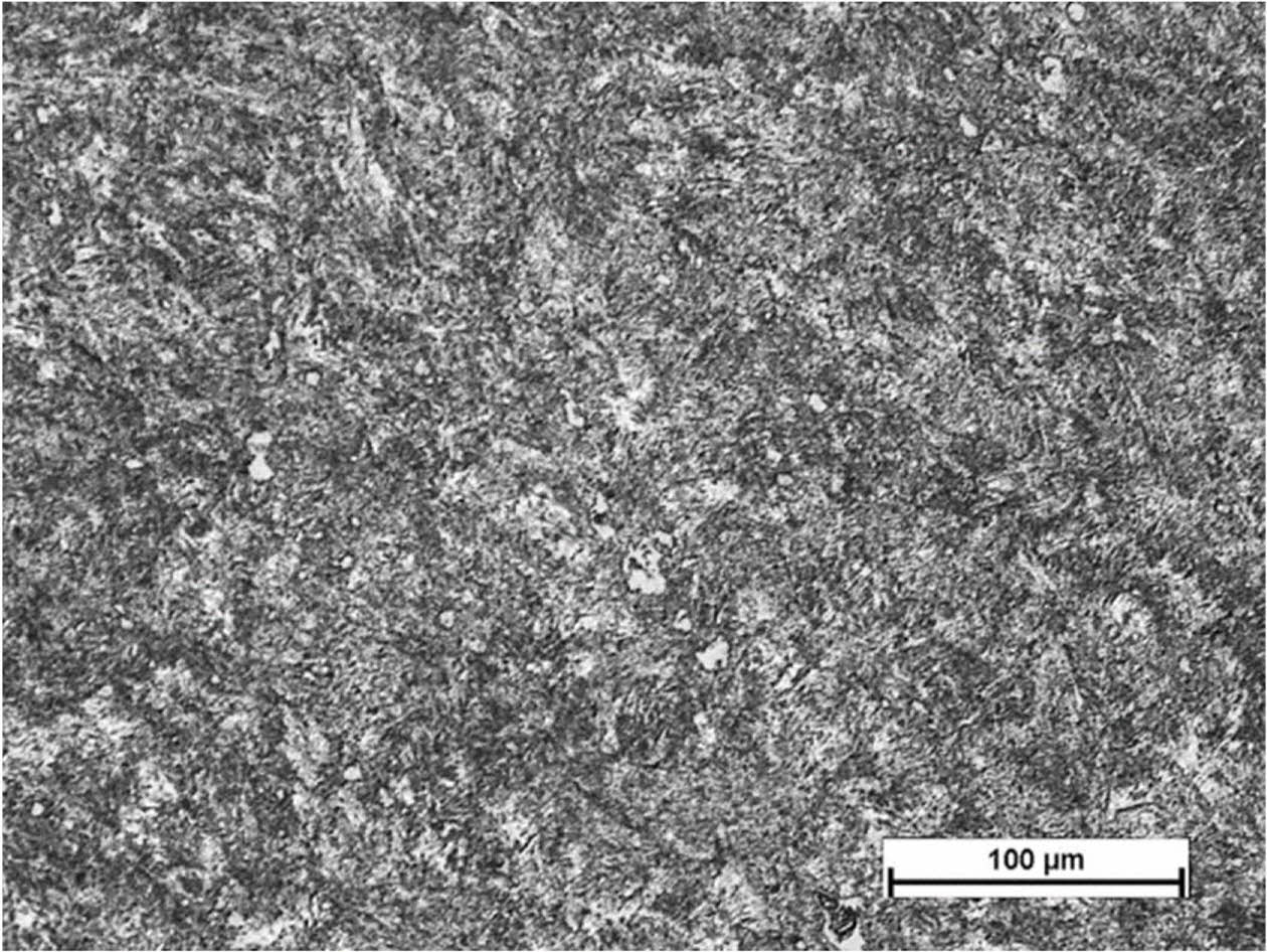
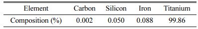
Titanium is lighter in weight is very resistant to corrosion and in most conditions, it frequently surpasses the resistance to corrosion of stainless steel. Grade 2 is the alloy of preference for the majority of industrial purposes requiring strong ductility and resistance to corrosion of four practically pure titanium grades. Titanium Grade 2 has a reduced density which makes it highly desired for weight. The strength and excellent corrosion tolerance of titanium grade 2 also makes it suitable for use in chemical, marine and desalination applications [13]. Oil and gas components, reaction and pressure vessels, tubing or pipe systems, heat exchangers, flue gas desulfurizing systems, and many other industry components are often utilizes Grade 2 titanium alloy. This grade 2 alloy at normal temperature behaves like an alpha alloy but transforms at 913±15 ^oC to beta phase and again returns back to alpha phase upon cooling below [14]. The density of grade 2 alloy is 4.51 g/cc with 103 GPa elastic modulus and 11.4 W/m^oC of thermal conductivity, hardness of 145 HV, 448 MPa and 344 MPa of yield and ultimate tensile strength. Table 1 presents the elemental composition of titanium grade 2 alloy and SEM micrograph is presented in Fig. 1.

Reciprocated Travelling WEDM
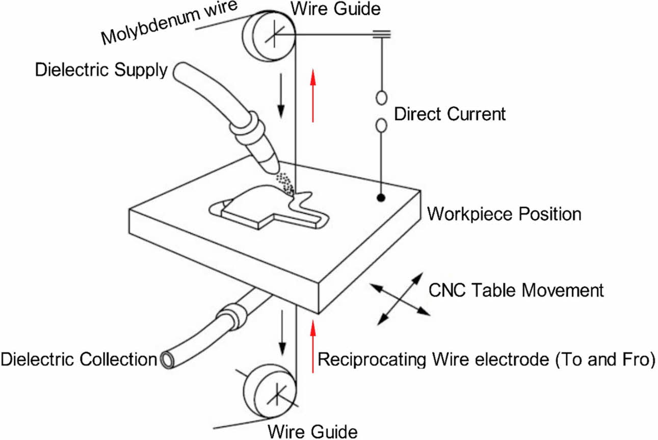
CNC WEDM machine releases impulse voltage towards workpiece and wire electrode through the sources that is controlled by the servo arrangement, to achieve a specific gap, and then discharges impulses in the fluid medium across workpiece and wire electrode [15]. As a result of the degradation of impulse discharging, a large number of small holes develop, giving the workpiece the desired shape. The cathode of the impulse power source is connected to the wire electrode and the anode of the impulse is connected to the workpiece. When the workpiece approaches the wire electrode in the dielectric fluid as the spark gap gets reduced to a definite value, dielectric liquid is broken through; very quickly forming a discharge channel and occurs an electrical discharge which releases extreme temperatures higher than 10000 ^oC instantly and the workpiece that is eroded cools down quickly under the influence of dielectric fluid and is flushed away [16]. Fig. 2 shows a schematic representation of reciprocating type WEDM where the molybdenum wire moves in to and for motion during the machining process.
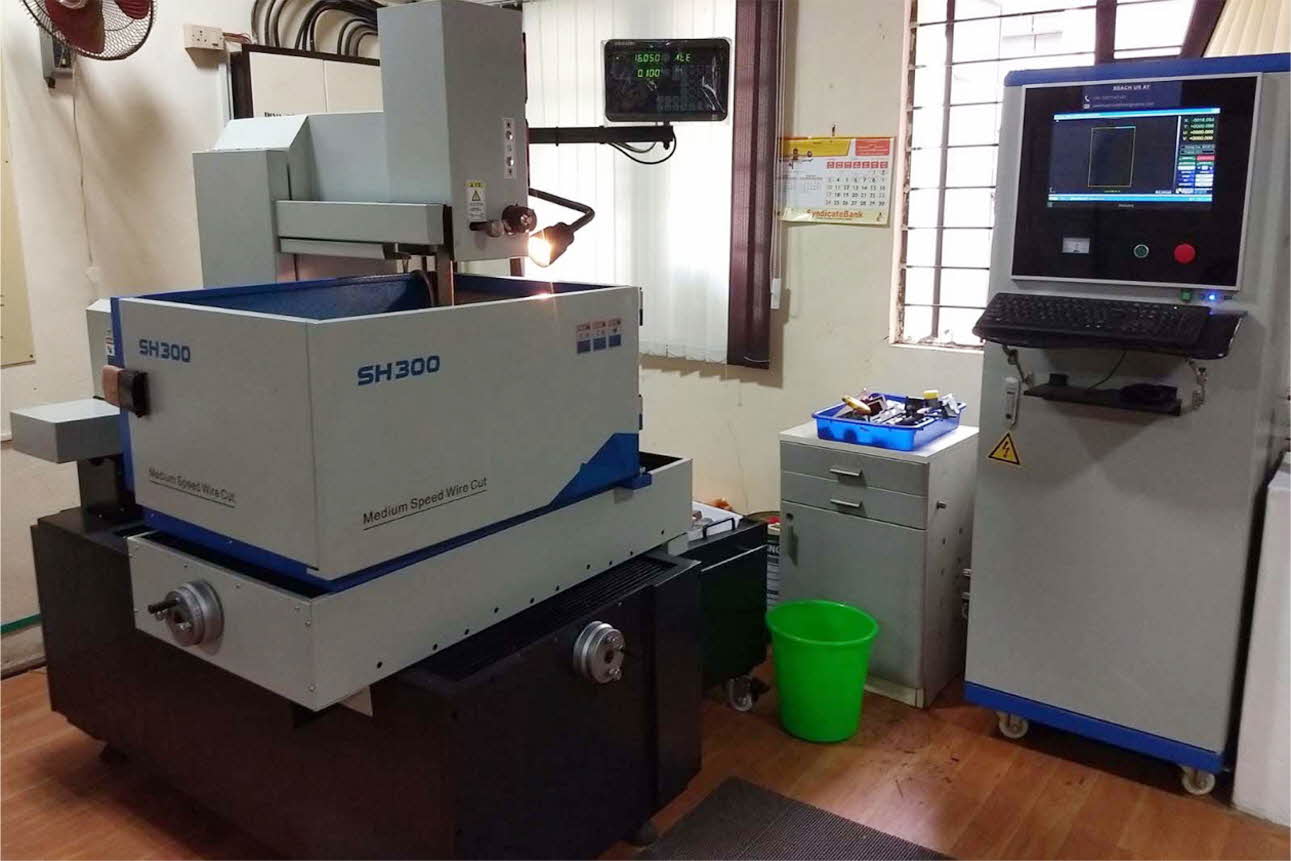
In high speed Wirecut electrical discharge machining (HS-WEDM) normally molybdenum wire electrode is used for high velocity reciprocating wire movement with a speed of 8-10 m/s. although the wire electrode is reusable thereby saving the consumption of molybdenum electrode, it produces lower accuracy and hence it is normally used in machines for domestic cutting [17]. The quality and speed of the process lies in between slow and fast WEDM and hence it is called as medium WEDM (MS-WEDM) which is an upgraded version of HS-WEDM which can machine multiple periods. As a result, its throughput is comparable to that of fast-moving WEDM, while its working quality is similar to that of slow-moving wire [18]. The WEDM-MS has greatly improved the shortcomings of the original WEDM-HS processing quality on the basis of the characteristics of simple structure, low cost, good process effect and low consumption in the process [19]. Fig. 3 presents the photographic view of RWEDM (MS-WEDM) setup used in this work consisting of electronic control panel, tank where the workpiece will be positioned and the dielectric is supplied and the table that can be fed in both transverse and in longitudinal direction.
The specification of SH-300 model RWEDM CNC machine is: Table travel of 300´400´250 mm, table size 550´680 mm, max workpiece weight of 350 kg, max cutting taper/angle of ±3^o / 80 mm, wire diameter of 0.16-0.20 mm, repeatability of ±0.003 mm, power capacity of 3KVA with pure water as working solution.

Molybdenum wire electrode
Molybdenum is an element that shares many pro- perties with tungsten that are extremely hard, higher melting point 2620 ^oC that features better thermal and electrical conductivity [20]. But unlike tungsten, it has greater ductility and a lower density. Molybdenum wire electrode consists of 99.97% pure molybdenum with a maximum carbon content of 0.01%. These wire electrodes are characterized for their super extension strength, excellent resistance to corrosion and oxidation in harsh corrosive and heat conditions. These wires develop high precision and are stable during cutting operation and hence its wont fracture easily and has higher life span. In WEDM these electrodes offer higher strength in tensile with lower elongation and has good precision and stability [21]. 0.18 mm is the wire diameter used during the experimentation.

Taguchi’s Experimental Design
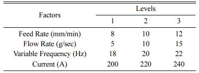
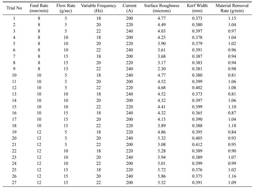
Taguchi employed orthogonal arrays (OA), which are a matrix of numbers organized in columns and rows to plan his experiments [22-27]. Each column gives a unique component whose influence on process capability can be evaluated, and each row indicates the levels (or conditions) of the evaluation criteria in a given study. The following syntax is commonly used to express an OA: L_a(b^c), The set of experimental runs is a, the quantity of variable combinations is b, and the number of array columns is c. The 'L' sign denotes that the data is structured on a Latin square factor arrangement [28-30]. Three parameters with three level values are investigated in this study, whereby a L₂₇(3¹³) OA was chosen and experimental design matrix is formulated [31]. A L₂₇ OA consists of 13 columns, in which columns 1, 2 and 5 is considered for formulating the experimental table. L₂₇ OA is selected to perform higher experimental investigation and to obtain higher output datasets so as to reduce experimental errors [32, 33]. Table 2 lists the control variables used in the machining studies, along with their values which are selected based on the literature and machine specifications.
The output responses considered are average value of surface roughness (Ra) measured on the workpiece surface after machining, kerf width (KW) obtained during machining and rate of material removal (MRR). Ra is calculated using the Mitutoyo Surftest SJ-210, which has a measuring span of 17.5 mm (X axis) and 360 m (Z axis) with 0.25 mm/s of measuring speed along with gaussian filter and 0.75 mN measuring forced and a cut-off of 0.08 mm. KW is determined by using optical microscope which is roughly twice of wire offset added with wire diameter. MRR is determined based on the formulate provided in Eq. (1) [34].



Technique for Order of Preference by Similarity to Ideal Solution (TOPSIS)
Hwang and Yoon [35] established Technique for Order Preference by Similarity to Ideal Solution (TOPSIS) predicated on the assumption that preferred option should be the furthest from the optimum alternative and the furthest from the negative-perfect solution. Consider that every factor has a monotonically rising (or declining) utility; then it's simple to find the “optimal” solution, which is made up of all possible greatest attribute quantities, and the “negative-ideal” solution, which is made up of all possible worse attribute values [36, 37]. In a geometrical perspective, one technique is to choose an option that has the (weighted) shortest Euclidean distance to the optimal solution [38]. The TOPSIS technique assesses the decision matrix below, which has “m” options and “n” variables:



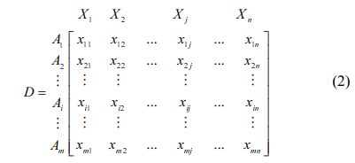
Here, A_i is the considered i^th alternative and the outcome of that alternate is x_ij as concerned with j^th condition. TOPSIS technique is done in a systematic procedure.

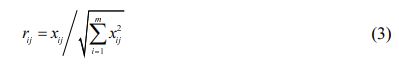
Step 1: Establishing Normalized Decision matrix:
This practice aims to alter the numerous attribute dimensionality into non-dimensional qualities so that they can be compared. One method is to split every criterion's result by the average of the overall outcome vector of the condition in question [39]. The normalized decision array R's element r_ij could be computed as:



Subsequently, every component has the similar vector unit length.

Step 2: Establishing the weighted normalized decision matrix:

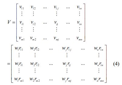
Weightages 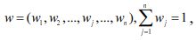provided by the person making the decision is included into the decision matrix. By multiplying the matrix column R with the provided w_j this matrix can be obtained. As a result, the weighted normalized decision matrix V equals:



Step 3: Finding the negative and positive ideal values: Let's define the two alternatives A^* and A^- as follows:



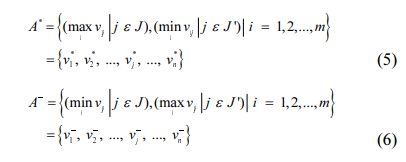
where J ={j =1,2,...n|j} associated with gainmeasures and J' ={j =1,2,...n|j}related with cost measures. Then it's safe to assume that the two produced alternatives A* and A- represent the most desirable (ideal solution) and less desirable (negative-ideal solution), correspondingly [40].

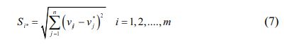
Step 4: Separation measure calculation:
The n-dimensional Euclidean distance can be used to calculate the distance among each choice. The distance between alternative and the ideal one is then calculated as follows:



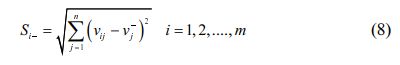
Correspondingly, the distance from negative-ideal value is



Step 5: Determination of relative closeness towards ideal value:
The value of A_i towards relative closeness regarding A^* is given as:



It is obvious C_i*=0 if A_i=A^- and C_i*=1 if A_i=A^*, alternate value of A_i is nearer to A^*when C_i*values approach towards 1.

Step 6: Ranking the order of preference:
As per the values of C_i* sorted out in descending order alternatives are ranked as per the preferences accordingly [41, 42].

Particle Swarm Optimization
The second population-based approach influenced by animals is particle swarm optimization (PSO) [43]. In that the PSO is not used by mutations/crossover pheromones or operators, it is analogous with ant colony or genetic algorithms, but significantly simpler. Rather, it depends on global communication on randomization of real numbers and swarm particles. This algorithm adjusts the paths of discrete units, termed particles, as piecewise ways created by positional vectors in a quasi-stochastic mode to explore the region of an objective function [44]. The technique is based on two fundamental concepts: coordinates and velocities for individual particle. In the solution region, individual particles have an initial velocity and a coordinate.
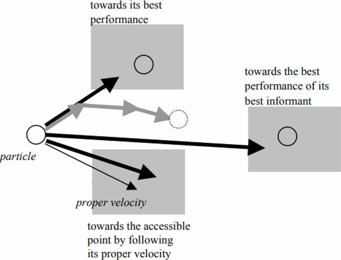
The particle updates itself to the current best when it locates a place that is better than the previously identified location. At any point throughout iterations, there's also a current best for all particles. The aim is to seek the global best solutions until the objective is no more improvement or a number of iterations have been finished. The particles advance toward the optimal solution locations as the programme advances. PSO takes less storage and has no operator because it is so easy to accomplish [45]. PSO is a quick algorithm due to its simplicity. Fig. 4 shows a graphic representation of particle movement in PSO which tends to move towards the best position by varying its velocity towards achieving the optimal position or condition. For the calculation of a particle's future displacement, three key elements are used: the particle's own velocity, its best performance, and best informant greatest performance. The three grey arrows represent a possible combination that will result in the particle's subsequent position [46].
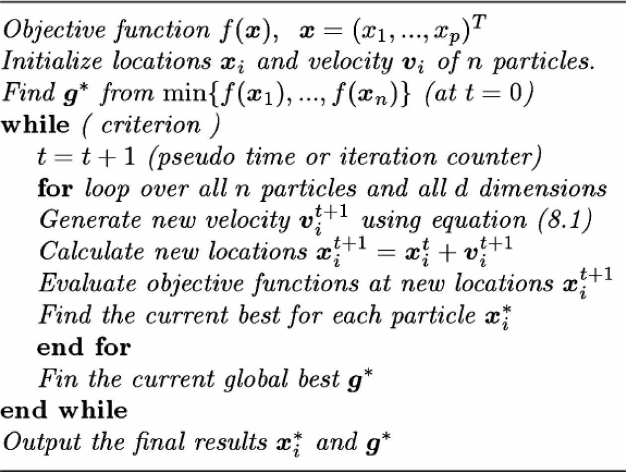
The basic procedure of implementing PSO consists of: (i) initializing PSO parameters, particles velocities and positions based on n-dimensional problem search space, (ii) compute particles initial local best positions and initial global best position using objective function, (iii) update each particles position and velocity, (iv) for each particle compute the objective functions, (v) update each local best particle using computed objective functions values, and (vi) update global best particle using computed local best particles objective functions values. The mainprocedures in PSO are summarized in pseudo code presented in Fig. 5.

With the designed experimental matrix (L₂₇ OA) machining is performed on RWEDM setup and the output responses viz., SR, KW and MRR are measured and recorded as in Table 3. Outcomes show that higher wire electrode rate of feed, SR and KW increases with decrease in MRR [47]. On contrary with higher flow rate of dielectric among the workpiece and non-utilizable electrode, higher MRR is obtained with lower SR and KW [48]. Increasing the variable frequency substantially increases the higher removal of material from the workpiece along with higher KW but a better surface finish is obtained. The influence of current on the output shows that with rise in current during machining MRR, SR and KW tends to lower [49, 50].
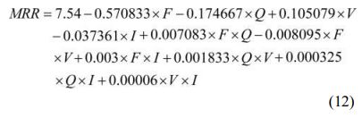
Further towards understanding the influence of input factors on the obtained responses, 3D surface plots are drawn. Fig. 6 presents the 3D surface graphs plotted among the SR and considered inputs. Higher rate of feed obviously increased the SR in a linear trend whereas higher flow rate of dielectric considerably reduces the SR in a linear manner. A linear relationship exists among the variable frequency and SR and also with current as it is represented by linear variation. Increasing the variable frequency lowers the SR but with increase in current SR tends to increase [51].
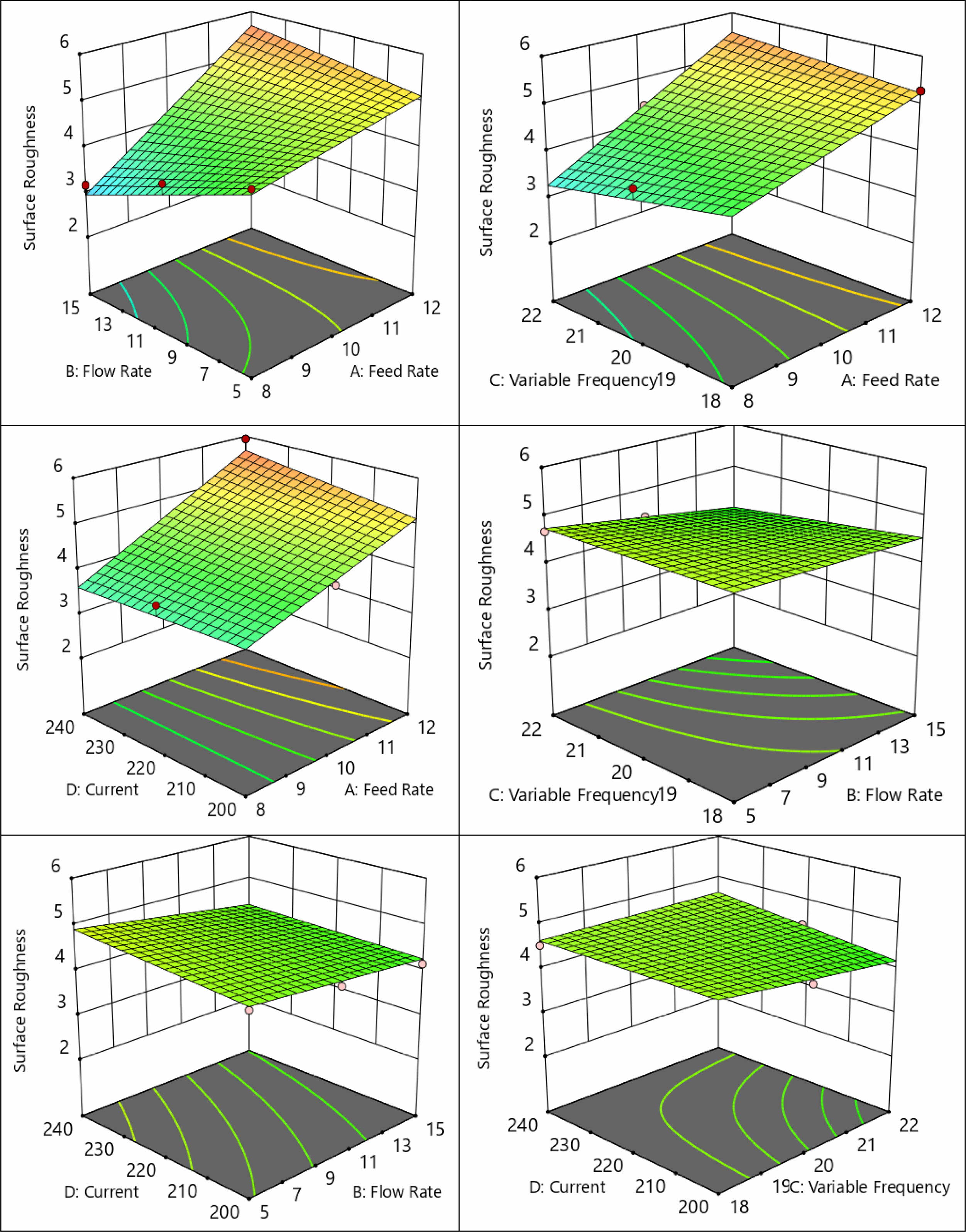
The surface plots of KW drawn to identify the relationship with different input parameters are shown in Fig. 7 which infers that with higher values of feed rate significantly increases the KW due to the higher spark density between the workpiece and wire electrode. Increasing the flow rate of dielectric increase the KW as the molten material that is removed from the workpiece is flushed away considerably. KW tends to increase with higher variable frequency due to the availability of higher spark density will eventually removes more material. A reduction in KW is observed with increasing current but higher KW is obtained for a combination of lower current density and higher variable frequency [49].
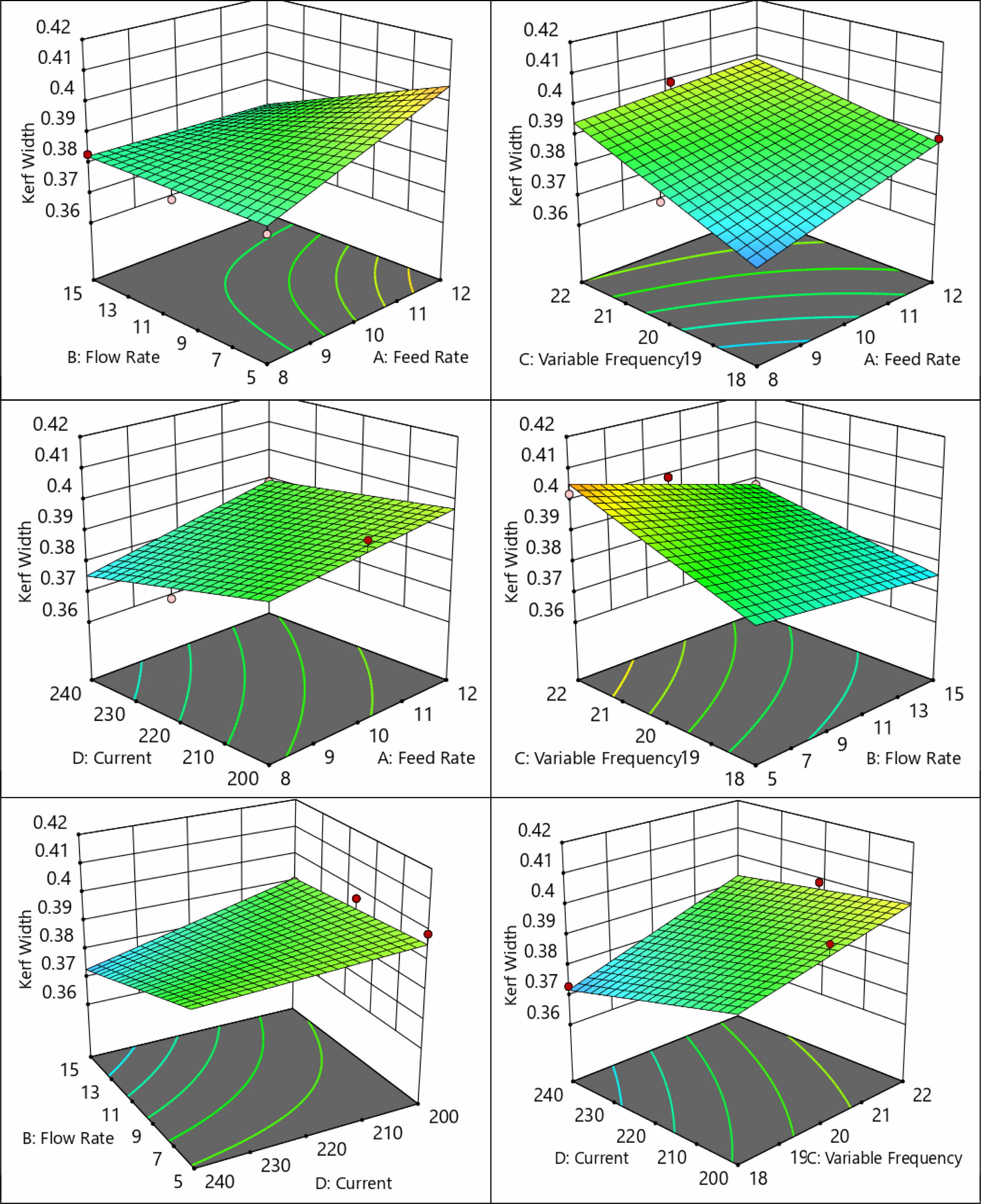
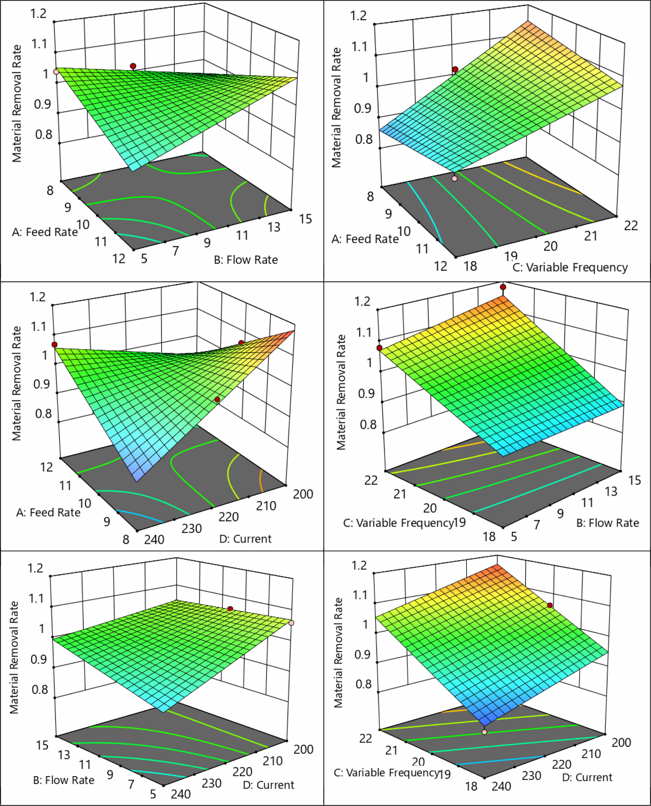
Fig. 8 presents the surface plots of MRR for different inputs, lower MRR is attained with increase in wire electrode feed rate as less material is eroded from the workpiece material. But with higher dielectric flow rate the MRR tends to increase significantly as the eroded material in molten state is flushed away considerably. Increasing the variable frequency obviously increases the time of spark which obviously increases the MRR. But higher current density lowers the MRR due to insufficient erosion of workpiece material; higher variable frequency and lower current produces higher MRR [52].
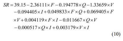
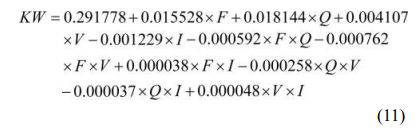
For the obtained output performance characteristics mathematical modelling is done for forecasting responses for the supplied input conditions with the considered lower and upper range of inputs. A non-linear second order model is generated for SR (Equ. (10)), KW (Eq. (11)) and MRR (Eq. (12)) using regression modeling technique [61]. The R² value obtained during model development is 90.72% for SR, 92.84% for KW and 93.74% for MRR.





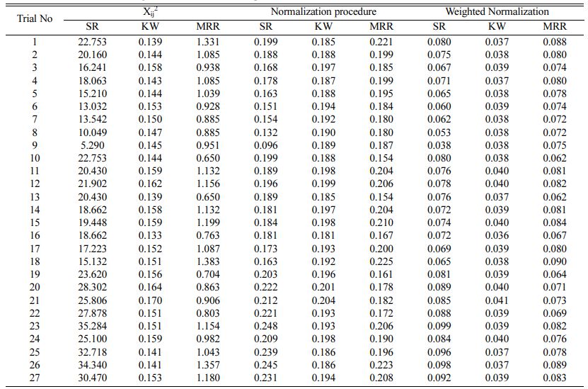
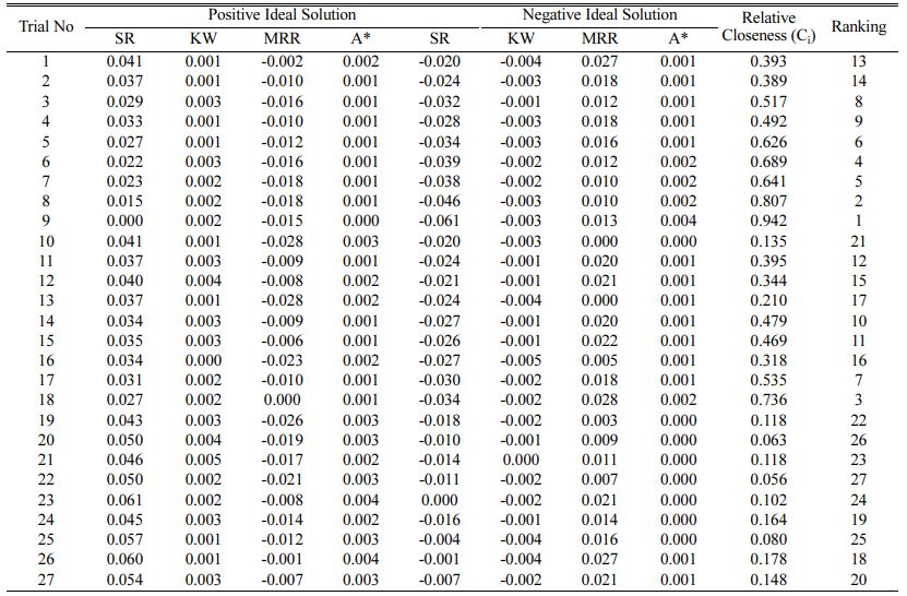
After mathematical model development, optimization is carried out for enhancing the RWEDM performance by simultaneously optimizing the SR, KW and MRR. This work minimizes SR and KW for better surface integrity and quality whereas maximizing MRR for achieving higher cutting speeds and productivity. For multicriteria optimization TOPSIS procedure is imple- mented. The first phase is to turn the outputs into a standard sequence (i.e., conversion of values within 1 and 0). Table 4 shows SR, KW and MRR data that are standardized between 0 and 1 and subsequently weightages are supplied to SR, KW and MRR after normalization method. Equal weightage (40%) is considered in this analysis towards SR and MRR whereas for KW 20% weightage is considered as more importance is given for surface integrity and productivity. On the basis of the eq. (4) provided, Table 5 shows the established positive optimal solutions (max for MRR and min for SR and KW) and negative ideal solution (min for MRR and max for SR and KW)obtained for SR, KW, and MRR. As per Eq. (8) the values of relative closeness (C_i) are determined for combined characteristics of SR, KW and MRR as displayed in Table 5. From the values of relative closeness grading is given as per the ideal values that are nearer to 1.
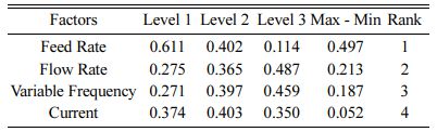
The next step towards optimization of considered input conditions over the multi-criteria characteristics is formulation of response table. By considering average values of relative closes corresponding to distinct factor values, formulation of response table is done as depicted in Table 6. The effect of the specified parameters may be determined from the grading given on the basis of the variance between the highest and minima that match the respective levels [54]. The best is ranked 1 and the lest significant is ranked 4.
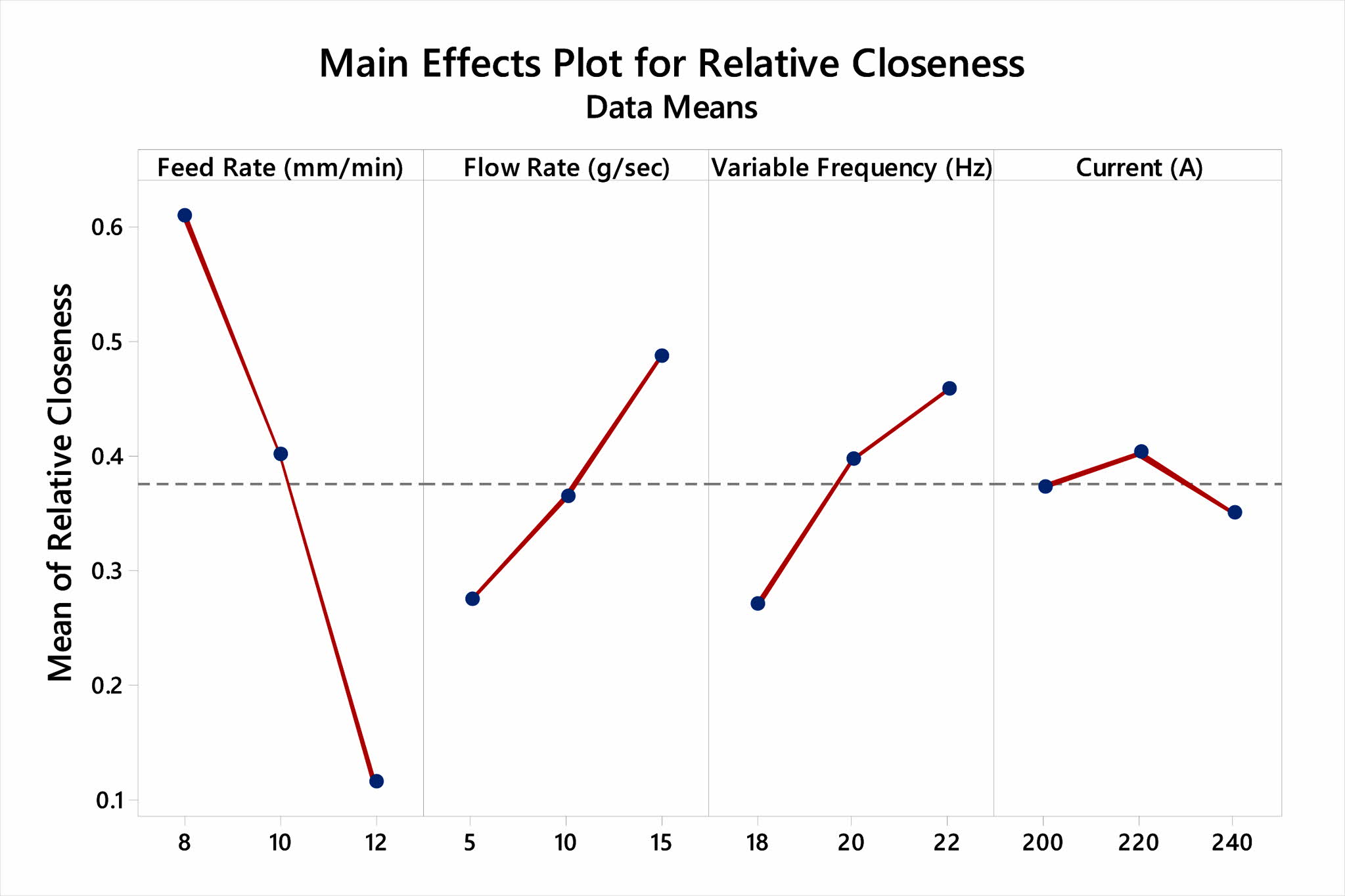
Based on the formulated response table, linear graph or main effects plot is drawn (Fig. 9) and the identified optimum conditions are 8 mm/min of wire electrode feed rate, 15 g/sec flow of dielectric medium, 22 Hz of variable frequency and 220 A of current density.
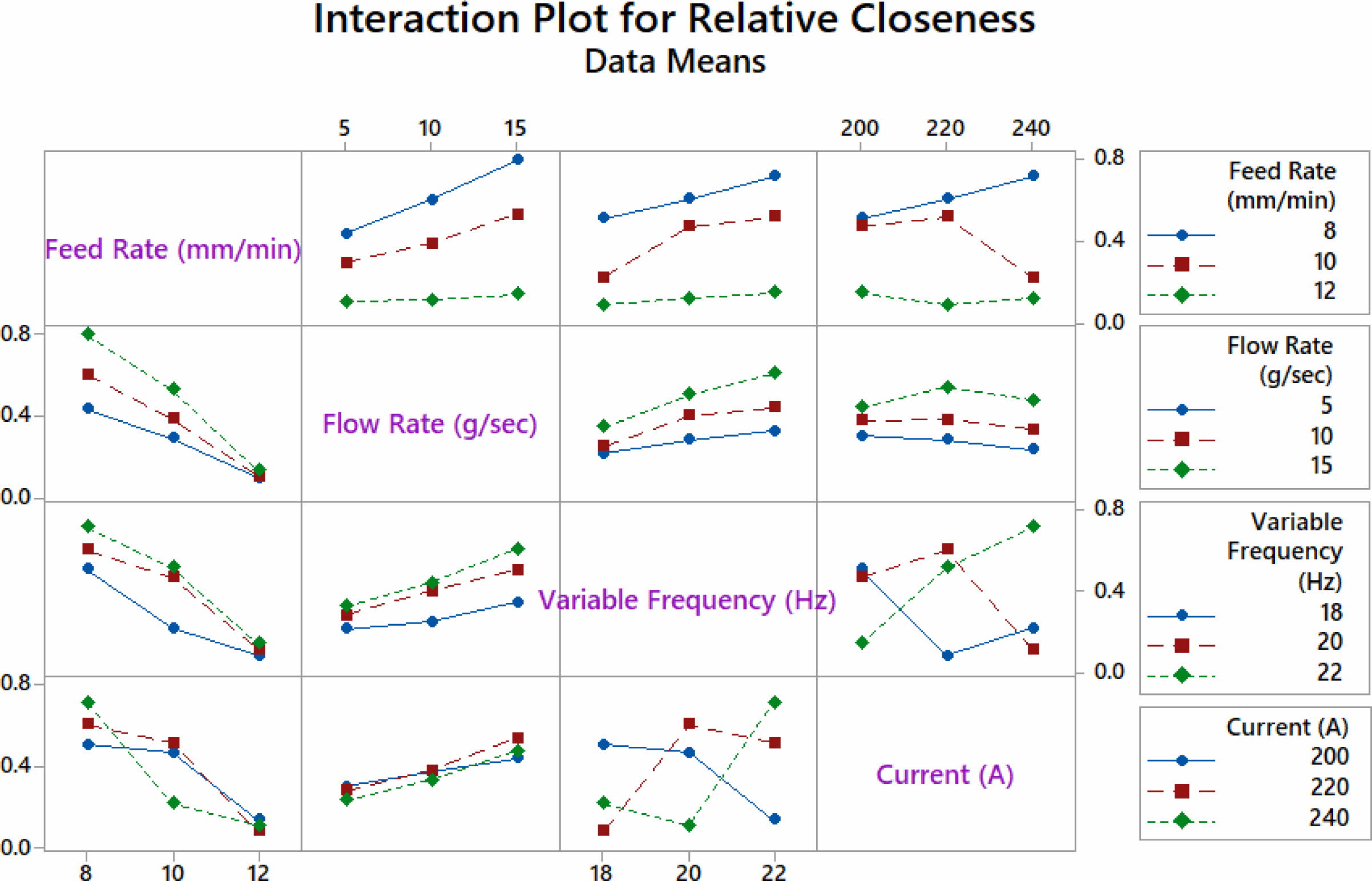
When planned experiments incorporate several factors, the potential for each component to interact with another one or more factors rises quadratically. This may be achieved through the effects of one factor [54] and another. Most of the times no combined impact between the components is experienced in the interaction chart when lines are comparable; when differences occur between two factors, a coexistence is across the variables. The more interactive the lines, the wider the distance between the components [24]. Fig. 10 shows the consequence of inputs on relative closeness during RWEDM of titanium grade 2 alloy. It is observed that no interaction is perceived among feed rate and flow rate and also between feed rate and variable frequency. But a moderate combinatory influence is observed among feed rate and current density. Similarly, no interaction is observed among flow rate and variable frequency and among flow rate and current density. A stronger interaction is seen between variable frequency and current as their relationship is represented by means of nonparallel lines.
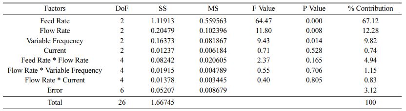
A statistical technique analysis of variance (ANOVA), used to analyze outputs based on several modules of effects that work simultaneously, to select important types of affects and to assess findings [55-57]. Table 7 depicts the ANOVA outcomes for relative closeness considering both main effects and significant interaction effects, with 67.12% contribution rate of feed of wire is the critical input trailed by flow rate with 12.28% contribution, variable frequency with 9.82% contribution and interaction between feed rate and flow rate contributing by 4.94%. The least contributing parameter is current density with 0.74%. The R² value obtained during analysis is 96.88% which is reasonably good as this procedure is carried out with 95% confidence interval [58].
After identifying the optimum input condition with TOPSIS, a non-traditional metaheuristic algorithm PSO is used for optimizing the RWEDM process parameters. Here also the prime objective is to lower the lower the SR and KW and to get higher MRR during machining, objective function is formulated based on the requirement as:
Objective function formulation: Maximize MRR + Minimize SR + Minimize KW.
Equal 40% importance is given to MRR and SR whereas for KW 20% importance is provided. Unconstrained optimization is done in this work with the considered constraints of parameters as:
8 ≤ feed rate ≤ 12
5 ≤ flow rate ≤ 15
18 ≤ variable frequency ≤ 22
200 ≤ current ≤ 240
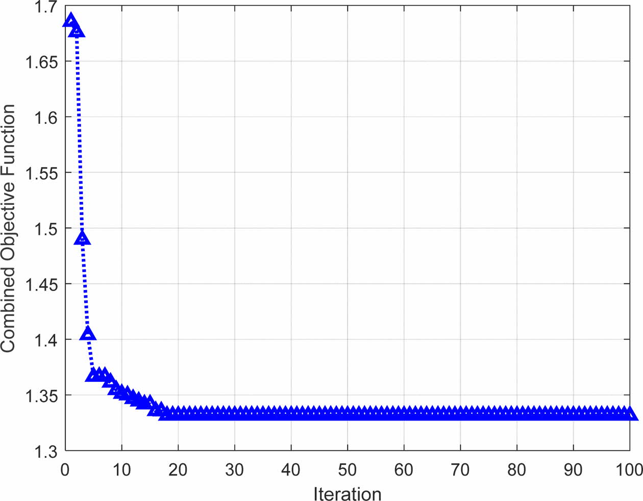
The optimum conditions of machining are determined from the simulation results using PSO; wire feed rate of 8 mm/min, dielectric flow rate of 15 g/sec, variable frequency of 22 Hz and current density of 210 A. The combined objective achieved for each repetition of imitation is offered in Fig. 11. Initially during execution of algorithm, the combined objective function value is nearer to 1.5065 and as the iteration continue, it converges at a faster rate at 10^th iteration itself to reach the optimum combined objective value of 1.3316.
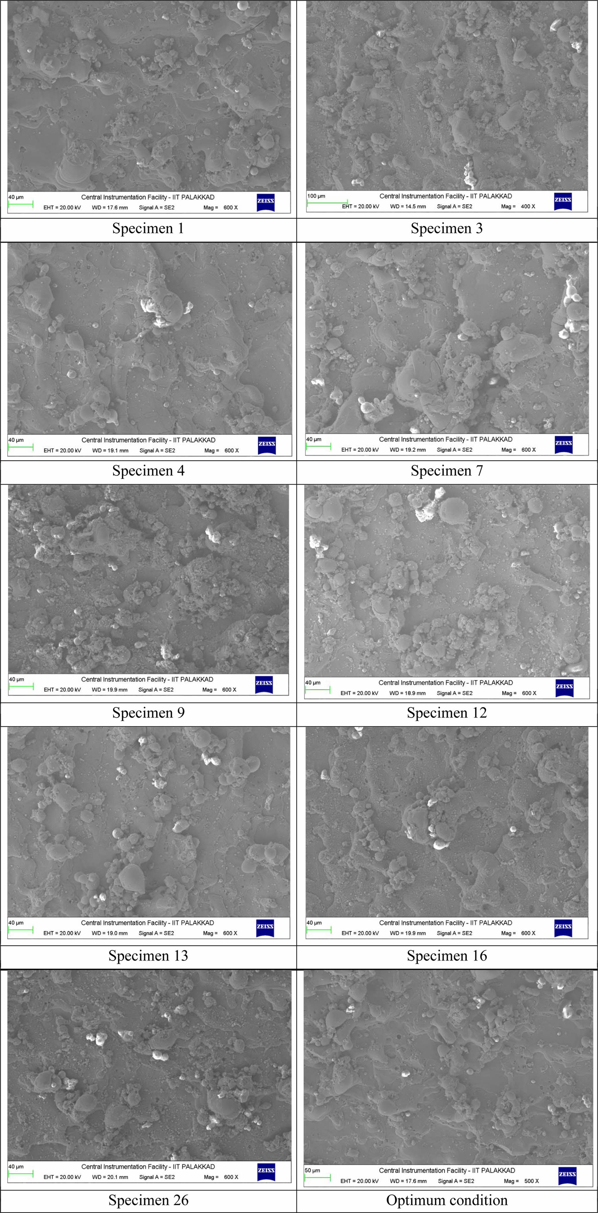
Fig. 12 depicts the SEM pictures taken from the workpiece surface for the analysis of the recast layer. The refurbishment layer consists of melted metal particles which have been placed on the workpiece's surface. Workpiece erosion can be visualized and melted materials are seen as clusters formed because of the solidification of the eroded materials. Higher current rises the discharge energy in the spark gap which accelerates melting and evaporation of workpieces. Due to higher temperature dielectric is unable to flush the eroded and melted materials which solidifies in the surface of machined workpiece [59]. Voids and micro- cracks might potentially include the HAZ and the recast layer, which could induce key component stress failures. Recast strands are unwanted, because they can be fractured and broken and variation in hole form and size can be introduced[60]. It is seen that the workpiece is less distorted and that the refurbishing layer is lower in thickness.
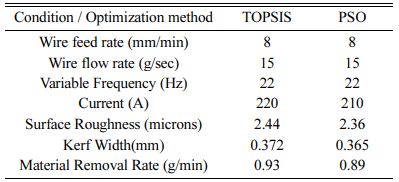
After recognizing optimal setting on the considered input parameters through TOPSIS and PSO, a validation experiment is performed in the RWEDM considered for study and the outputs obtained are tabulated in Table 8. As against the experimental trials, the outcomes of authorization experiment produce higher MRR is obtained with lower SR and KW.
From the comparison of outcomes from TOPSIS and PSO there is deviation of SR by 3.27%, KW by 1.88% and MRR by 4.3% which is close enough for better optimization conditions.

In this work, optimization and statistical analysis of RWEDM of titanium grade 2 alloy is performed using molybdenum wire considering wire feed rate, dielectric flow rate, variable frequency and current over the output responses viz., SR, KW and MRR. The outcomes of the present study are:
1. Outcomes from experimental analysis shows, with higher wire electrode rate of feed, SR and KW approaches to increase with decrease in MRR. On contrary with higher flow rate of dielectric among workpiece and electrode higher MRR is obtained with lower SR and KW.
2. Increasing the variable frequency substantially increases the higher removal of material from the workpiece along with higher KW but a better surface finish is obtained. The influence of current on the output shows that with rise in current during machining MRR, SR and KW tends to lower.
3. During analysis equal weightage (40%) is considered for SR and MRR whereas for KW 20% weightage is considered as more importance is given for surface integrity and productivity. The optimum condition obtained is 8 mm/min of wire electrode feed rate, 15 g/sec flow of dielectric medium, 22 Hz of variable frequency and 220 A of current density.
4. In order to study the combinatory effect, it is observed that no effect of interaction is perceived among tool feed and flow rate and also between feed rate and variable frequency. But a moderate combinatory influence is observed among feed rate and current density. A stronger interaction is seen between variable frequency and current as their relationship is represented by means of nonparallel lines.
5. ANOVA analysis presents that with 67.12% contri- bution, tool feed is the critical factor that influences higher continued by flow rate with 12.3% contribution, variable frequency with 9.81% contribution. The least contributing parameter is current density with 0.74%. The R² value obtained during analysis is 89.7%.
6. The optimum condition evolved from PSO are: 8 mm/min of wire electrode feed rate, 15 g/sec flow of dielectric medium, 22 Hz of variable frequency and 220 A of current density with a predicted SR of 2.36 microns, KW of 0.365 mm and MRR of 0.89 g/min. From the comparison of outcomes from TOPSIS and PSO there is deviation of SR by 3.27%, KW by 1.88% and MRR by 4.3% which is close enough for better optimization conditions.
7. From the recast layer produced it is observed that less distortion occurred in the workpiece and hence lower thickness of recast layer is seen here as the eroded and melted materials are properly flushed away by the dielectric.