Basic Oxygen Furnace (BOF), TBM type (Thyssen – Blas – Metallurgie)is one of the heat units occurring in a steel production process. The refractory lining of BOF consists of several zones and is lined with MgO-C bricks. For the above mentioned zones refractories with different properties are selected due to the different factors influencing the corrosion process. Intense wear of refractories is observed mainly at the slag spout zone in accordance to the influence of thermochemical, thermomechanical factors (including the oxidizing atmosphere).
The aim of this paper is to find the regression formula with satisfactory forecast measure of fit, which will make it possible to predict the refractory material wear in the slag spout zone of BOF depending on the real wear measurement made during the BOF operation. Calculations were conducted with the use of regression trees with CART algorithm (Classification and Regression Trees), Multivariate Adaptive Regression Splines (MARS), Boosted Trees algorithm and Multilayer Neural Networks MLP type (Multilayer Perceptron).Selected metallurgical parameters registered during the BOF campaign are the independent variables discussed in refractory material wear models, whereas the wear rate of refractory materials calculated per one heat is set as a dependent variable

Keywords: Basic oxygen furnace, Refractories, Machine learning, MgO-C

Basic Oxygen Furnace and Electric Arc Furnace are two heat units commonly used in the steel production process where at the beginning steel melt is prepared for the secondary metallurgy processes. In 2020 57,4% of crude steel produced in Europe was obtained from the Basic Oxygen Furnaces [1]. The refractory lining of such converters is made of high quality magnesia – carbon refractories. The designing process of lining is taken mainly due to the necessity of ensuring a safe and longest as possible operation time. Basic Oxygen Furnace campaign usually lasts for several months and the time of operation depends on the exploitation conditions and metallurgical parameters occurred during the campaign. The wear process of refractory lining is influenced by parameters like chemical composition of hot metal (Si, P, C, Mn, S content), hot metal temperature, temperature of melt at the end of the process, oxygen activity in the metal bath, chemical composition of slag etc. The main factors influencing the wear rate of MgO-C type refractories used for Basic Oxygen lining and overall issues concerning the corrosion of MgO-C materials lined in a steel metallurgy heat units are described briefly in [2-10] where authors additionally propose different material solutions for selected Basic Oxygen Furnace wear zones. Another important factor influencing the wear of the refractory lining at the beginning of the campaign are thermal shocks associated with a preheating stage and mechanical stresses, which occur during the test vessel rocks. Moreover, thermal shock occurs during the hot metal load into a converter. Recently, different techniques of lining conservations like gunning, slag splashing and slag washing were developed which help to provide longer operation time.
From the point of view of refractories users and manufacturers, it is important to have an opportunity to predict the wear rate of refractory materials depending on the factors/process parameters which could be controlled and observed during the converter operation. To assess how the process parameters influence on the wear rate of refractories it is possible to use the Machine Learning Techniques. The attempt to use Neural Networks for such assessment with analysing real exploration data was taken by Zelik et al. [11].
This paper is a continuation of analysis taken in [11] with use of an another Machine Learning Techniques described by Hastie et al. [12] including CART algorithm (Classification and Regression Trees), Multivariate Adaptive Regression Splines (MARS), Boosted Trees algorithm and Multilayer Neural Networks MLP type (Multilayer Perceptron).
Modelling the wear rate of the refractory lining of BOF was conducted on the basis of measurements of selected metallurgical parameters registered during its operation at the Steel Plant. There is no similar calculation in literature which would process different ML algorithms for predicting the wear rate of the slag spout zone refractories in BOF lining.
MgO-C material allocated for slag spout zone of Basic Oxygen Furnace.
In the slag spout zone high quality MgO-C refrac- tories are used. Such materials consist mainly of fused magnesia FM97.5 or FM98 type with mean crystals diameter > 1,000 µm, flake graphite content about 12 – 15% mas. As a binder liquid pitch is used. Parameters of the material which was installed in the converter and for which calculations are conducted are given in Table 1. This material is classified as MC95/10 in accordance to PN-EN ISO 10081 – 3:2006 (Classification of dense shaped refractory products - Part 3: Basic products containing from 7 percent to 50 percent residual carbon). This material is characterized by high corrosion resistance (including oxidation resistance), erosion resistance, excellent physical parameters (apparent porosity, bulk density).

Selection of parameters influencing the wear of the MgO-C type oxygen converter lining.
During the Basic Oxygen Furnace operation selected process parameters are registered, which make it possible to control the chemical composition of hot metal and parameters of processing liquid melt. Parameters which have a significant impact on the wear rate of refractories are as follow: Si, C content in hot metal, temperature and mass of hot metal, oxygen activity in metal bath, temperature at the end of the process, amount of oxygen used during the upper blow, amount of calcium added to the vessel, amount of additives which are the source of MgO, concentration of MgO, FeO, Al₂O₃, SiO₂ in slag. During the campaign the process of conservation (gunning, slag splashing, slag washing) is registered, but the procedure of this registration is still improving. Corrosion mechanism of MgO-C materials and mentioned above parameters with their impact on the converter’s durability are described in [13-17].
Industrial experience shows that 13 parameters have a particular influence on the MgO-C type refractories wear rate and were selected for analysis in this thesis: (X₁) hot metal mass [kg/heat], (X₂) hot metal tem- perature [℃], (X₃) C concentration in hot metal [% mas.], (X₄) Si concentration in hot metal [% mas.], (X₅) scrap mass [kg/heat], (X₆) amount of added calcium [kg/heat], (X₇) amount of oxygen O₂ in upper blow [Nm³/heat], (X₈) final temperature [℃], (X₉) oxygen activity [O] in metal bath [ppm], (X₁₀) MgO concen- tration in slag [% mas.], (X₁₁) slag basicity, (X₁₂) total Fe concentration in slag [% mas.], (X₁₃) amount of additives which are a source of MgO [kg/heat].

Initial data preparation
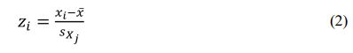
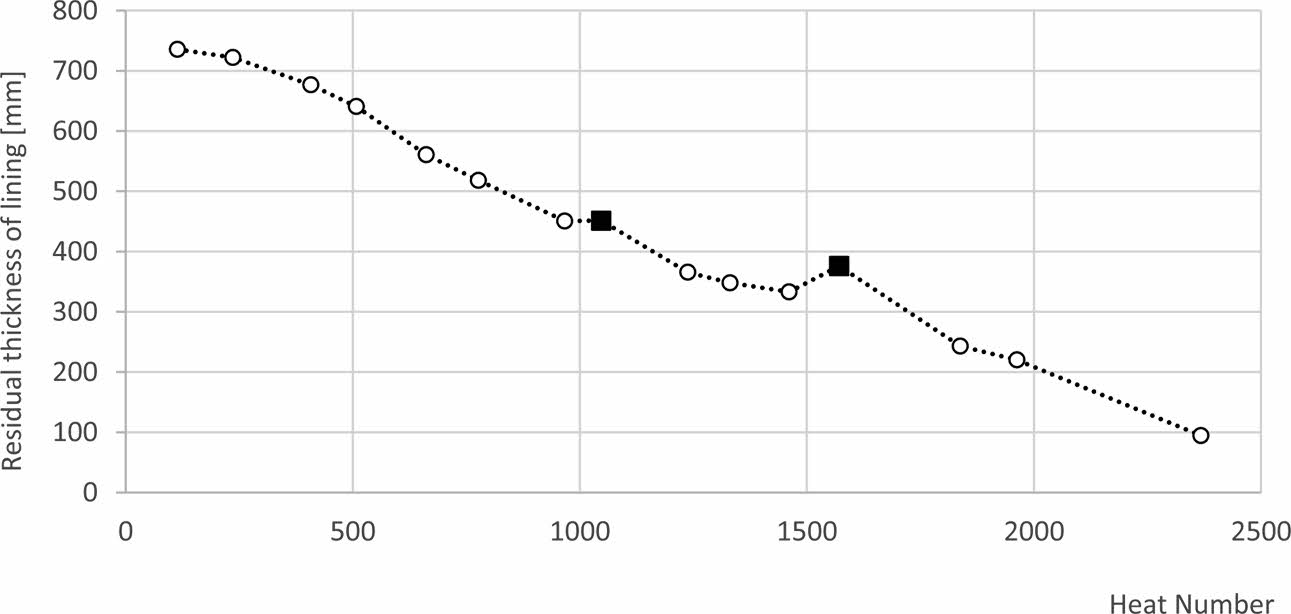
The wear rate of the refractory lining is measured by Steel Plant Staff with a help of a special laser device. The amount of measurements during the campaign depends on the production schedule and it is always about 15-20 measurements. The wear rate is determined by calculating the loss of the refractory material observed in a measurement period in relation to the number of heats realized in this period. That way the wear rate estimates the value of material lost calculated per one heat [mm/heat]. Fig. 1 shows the mean values of the residual thickness of the bricks from the left and right slag spout zone obtained from laser measurement. On Fig. 1 two points show that the thickness of lining increased heat after heat which is associated with residual slag stuck to the lining, residual gunning mixes or slag stuck to the lining after the slag splashing operation. In real conditions it is not possible to observe an increase in the lining thickness. For this reason two mentioned above points were substituted by interpolation based on the linear trend assumed across the entire campaign.
Linear interpolation was conducted with the use of Time Series and Forecasting Module provided by Statistica 13.3.software. Values which show residual thickness increase were deleted and substituted by values forecasted on the basis of linear trend, which is shown in Fig. 2. In this method algorithm fit the linear trend function to time series with the use of least square method.
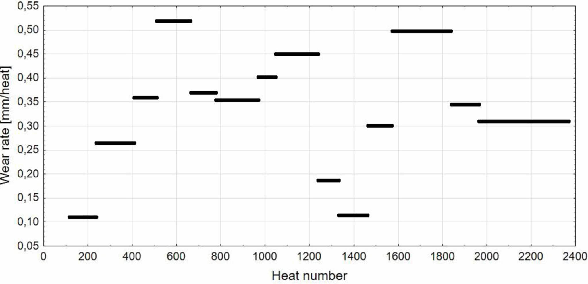
Basing on laser measurement of lining residual thickness, the wear rate of the refractory lining was calculated per one heat. The campaign was finished after 2386 heats. In calculations conducted in this paper first 114 heats were not taken into consideration due to an abnormal lining wear associated with thermome- chanical rather than thermochemical factors. Last 20 heats were not taken into consideration too because of not conducting the measurements by the steel plant staff. It is an usual practice when coming to the end of campaign an intense wear of lining can be easily seen and visual assessment of lining condition is enough to come up with the decision of taking out the heat unit from operation. Finally, data from 2252 heats was taken into analysis. The calculated wear rate was assigned to every heat from the measurement period. For example when measurement was taken after 150 heats then calculated wear rate was assigned to heats number 1-150. The wear rate after assignment to its period is shown in Fig. 3.
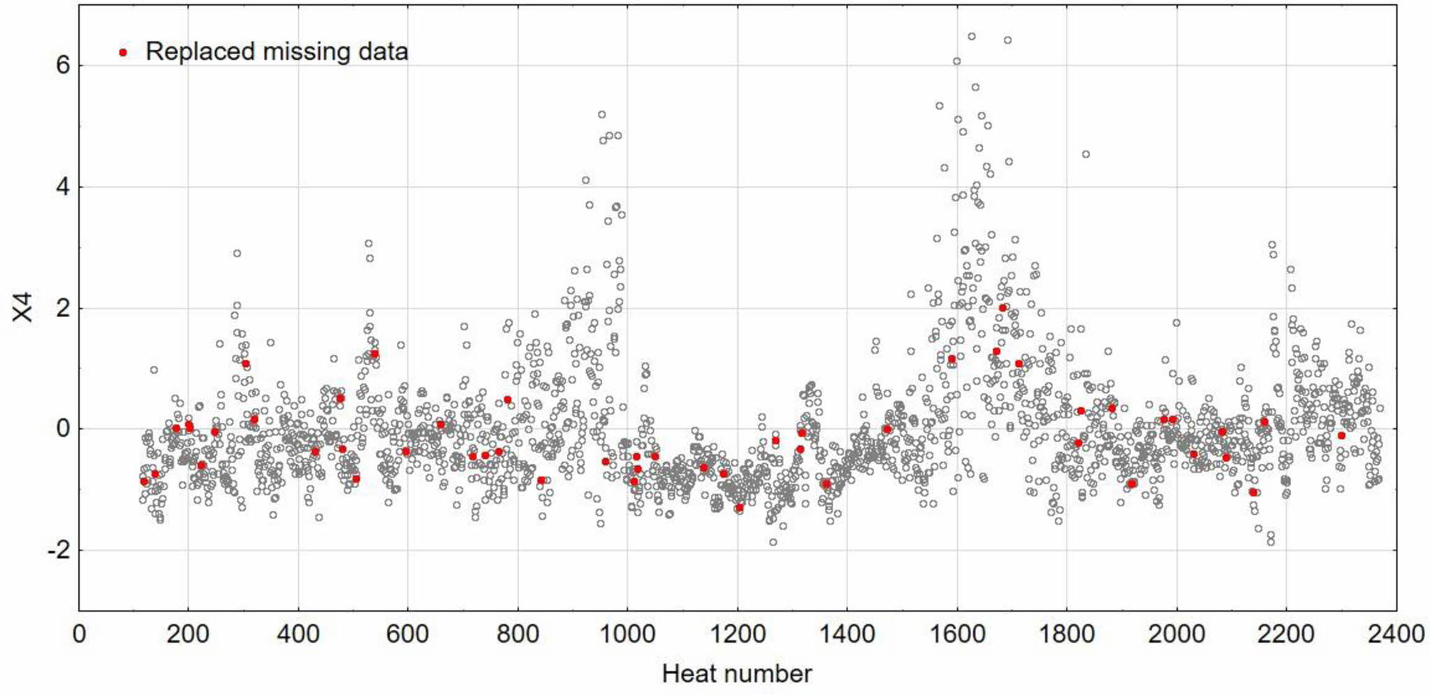
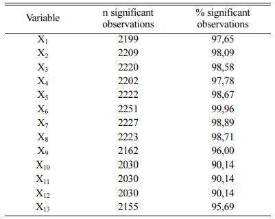
Data collected from the analysed campaign contains of missing values and data which should be deleted because of its unreal values (ex. amount of scrap and hot metal excessing vessel capacity), values equal “0” are deleted too. The contribution of significant values in the data set before replacing missing values is shown in Table 2. The initial data preparation was conducted with the use of R language and Statistica 13.3. software. The missing values were replaced with the use of Time Series and Forecasting Module form Statistica 13.3 software. The missing values were replaced using interpolation based on neighbouring non-missing points. The graphical method can be explained as connecting with a straight line the point located directly before and the point directly after the point with a missing value. The method assumes occurrence of autocorrelation in the data set when each observation is similar to the previous one. Si concentration in hot metal (X₄) with its standardized values and points with replaced missing data is shown in Fig. 4.
After replacing missing values, data smoothing for every variable was taken. The model of simple exponential smoothing was chosen with smoothing coefficient α = 0,2 calculated by formula (1) [18]:



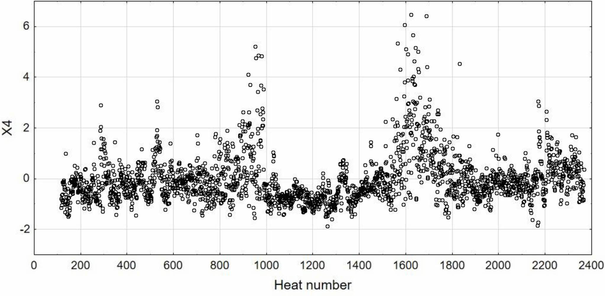
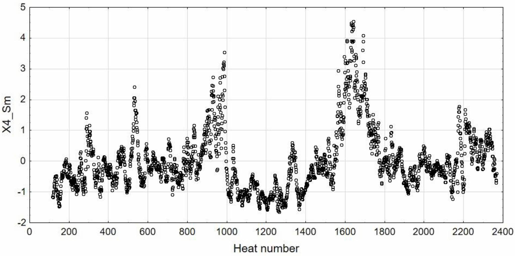
where: y_t is value of independent variable at the time t, γ̂_t – its forecast at the time t (smoothed value), α – smoothing coefficient as a weight for calculated weighted means. Smoothed value γ̂_t+1 at the time t+1 is a weighted mean of last observation with weight α and its prediction with weight 1 – α. Smoothed value (predicted) at the time t+1 is as sum of predicted value at the time t and fraction of previous prediction error value u (y_t + γ̂_t). As a result of the described procedure each observation from smoothed time series is a mean value of all previous observations when weights decrease exponentially. If α = 1, then smoothed time series is the same as the observed series. If α = 0, then series is constant and equal to initial observed values. For this reason α should be chosen from range 0 < α < 1. In this analysis smoothing coefficient α = 0.2 for provide smooth reaction of prediction values for variability of independent variables. Examples of data before and after smoothing are shown in Fig. 5-6.
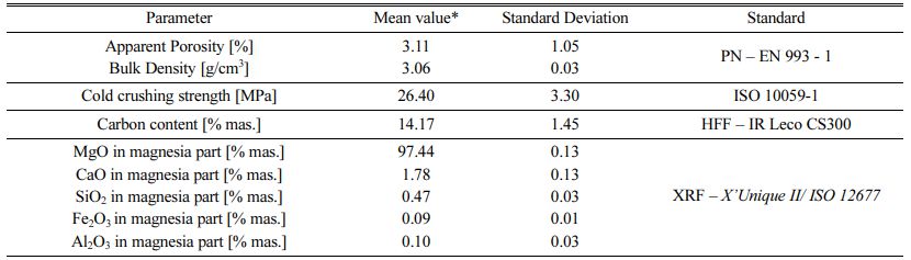
After smoothing the data values were standardized according to Formula 2 (2):



where: z_i – standardized value of independent variable X_j, where j = 1, …, 13, x – mean value of X_j, s_Xj standard deviation for variable X_j.

Model construction
Before setting up the model parameters, initial data set was divided to testing and training data with pro- portion equal 7:3. The proportion of testing and training data was estimated by the matter of trial and error till achieving the best model quality measured by different measures of fit further described. The calculation was conducted with the use of Statistica 13.3. software.
Parameters for building CART model were set as the following: minimal cardinality of nodes: 3% of entire number of measurements, maximal number of tree levels: 12 and n of child node: 10 (minimal cardinality of node created as a result of division).
Parameters for building the MARS model: maximum amount of basis function equal 90 (maximum amount of function which can be taken into the model before being cut). Interaction level: 3 and penalty for adding additional function to model: 2. Above mentioned parameters were estimated by the matter of trial and error to achieve the best model fit.
Parameters of Boosted Trees: number of analysed trees necessary for building the model: 500, minimal cardinality of nodes as 5% of entire number of mea- surements, maximal amount of tree level: 10 and maximal amount of nodes: 8.
MLP Network parameters: number of neurons in hidden layer: 2-10. As an error function SOS (sum of squares) between set values and output of network was chosen as a recommended for regression issues. Than function was chosen as an activation function for hidden neurons and linear function for output neurons. 20 networks were set up before the training process and for further investigation algorithm chose only 5 of them with the best quality measured by correlation coefficient between dependent variable and its prediction made by network.

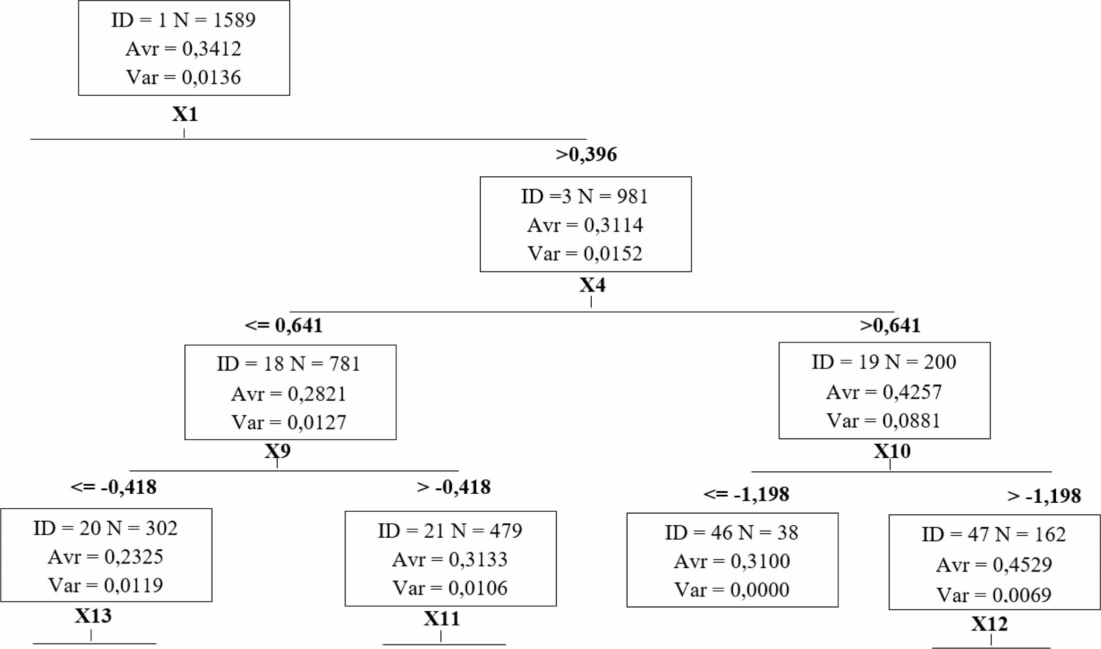
Using CART algorithm the tree with 24 divided nodes and 25 terminal nodes was obtained. Variable calculated as a root of tree was hot metal mass (X₁) which is shown in Fig. 7.
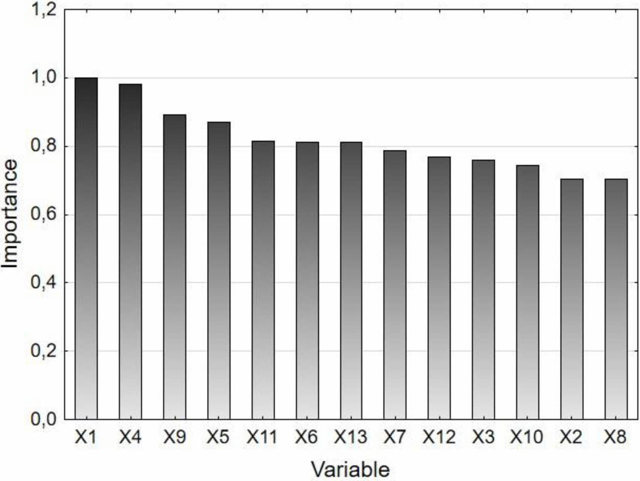
The influence of selected independent variables on modelling the response function can be assessed by the generation of importance plot shown in Fig. 8. The importance plot is generated as a result of multivariate analysis of impact of each independent variable on increasing the model quality, setting for every calculation step a different independent variable as an initial point of division. Values of the importance rate for increasing the model quality obtained from each independent variable are summed up in nodes and scaled towards the independent variable which acts most effectively. The independent variable with the most significant impact on changing the value of response function has range with value equal 100. CART algorithm found Si concentration in hot metal (X₄) as the most significant variable. Other variables with significant importance are: scrap mass (X₅), amount of added calcium (X₆), oxygen activity in metal bath (X₉) and hot metal mass (X₁).
In MARS algorithm a model with 65 factors and 150 basis functions was obtained. Complexity of this model makes it difficult to show regression equation and it will not be shown in this paper. After analysing several initial model parameters, the model with the lowest GCV = 0,004641 (Generalized Cross Validation)criterion was finally obtained. The coefficient of determination was R² = 0,71 and its adjusted value is R² = 0,70. By significantly expanding the prediction equation, it is possible to increase the quality of the model, but then the equation becomes not practical in use. The model most often refers to basis function for variables: hot metal mass (X₁), amount of added calcium (X₆), Si concentration in hot metal (X₄) oxygen activity in metal bath (X₉), scrap mass (X₅) which is shown in Table 3.
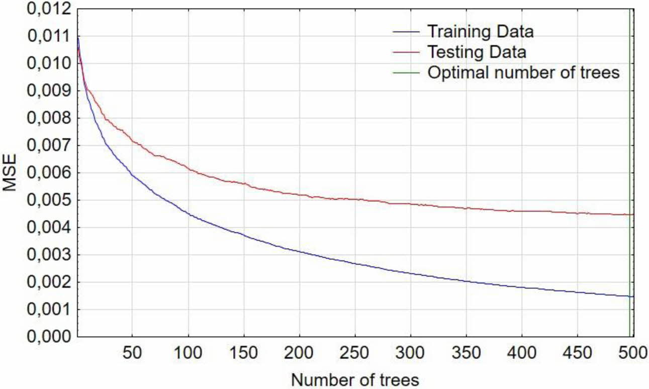
In Boosted Trees method, the number of trees necessary to build the model was set for 500. The optimal number of trees is chosen by the software automatically on the basis of errors occurring in the training data set, which values are shown in Fig. 9. There is no effect of overlearning observed during the training process which is characterized by spreading the curves describing mean square error in training and testing data. The optimal number of trees was calculated as 490 and was used for further calculations.
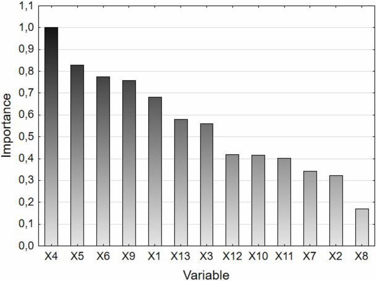
Similarly to CART algorithm, importance plot was generated and the most significant variables are: Si concentration in hot metal (X₄), oxygen activity in metal bath (X₉), hot metal mass (X₁), scrap mass (X₅), amount of added calcium (X₁₁) which is shown in Fig. 10. 5 most important variables estimated both in CART and Boosted Trees algorithm are: hot metal mass (X₁), Si concentration in hot metal (X₄), scrap mass (X₅), oxygen activity (X₉).
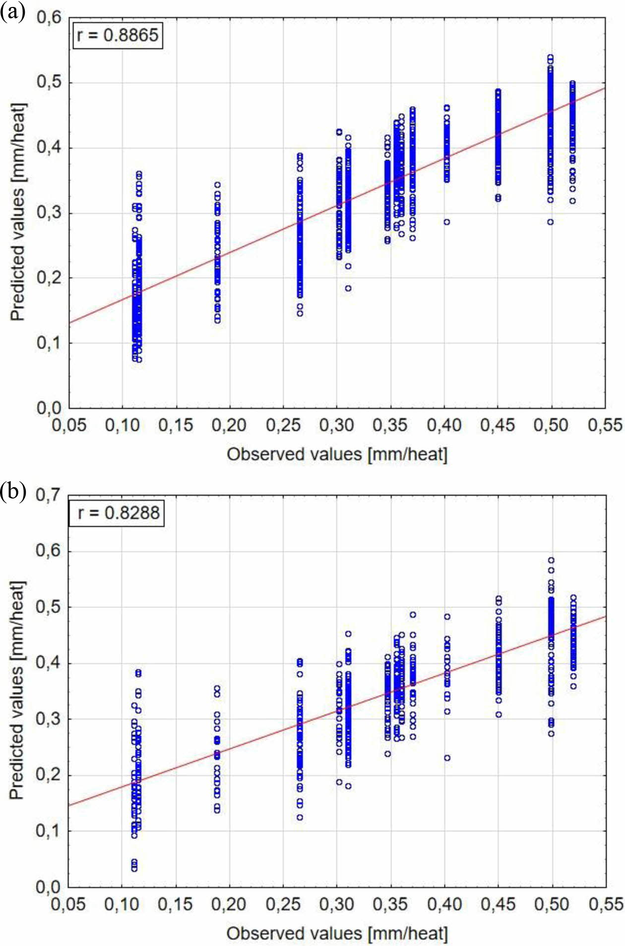
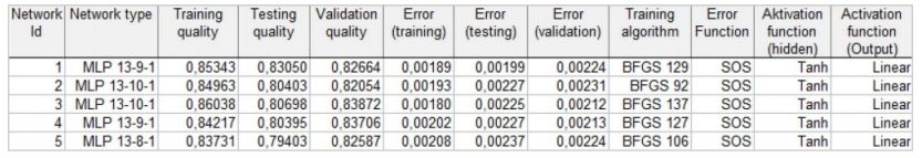
Topology of 5 active networks obtained from cal- culations are shown in Table 4. Networks differ by the quality of the training and testing process which depend on the numbers of hidden layers and number of neurons included in layers. Each of the selected networks contain 13 neurons in the input layer and from 8 to 10 neurons in the hidden layer. In Table 4 in the column “Training algorithm” the algorithm type and number of epochs used in the training process are shown.
In the analysed case more than one active network is obtained. It is possible to calculate a prediction for a group of network where a prediction is calculated as a mean value from every single prediction obtained from active networks.
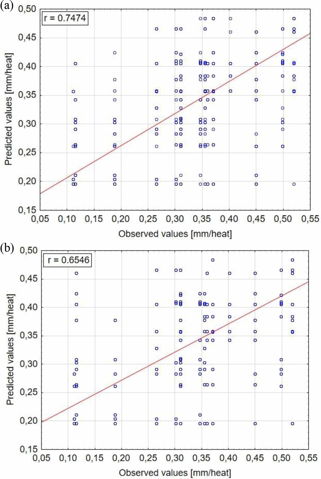
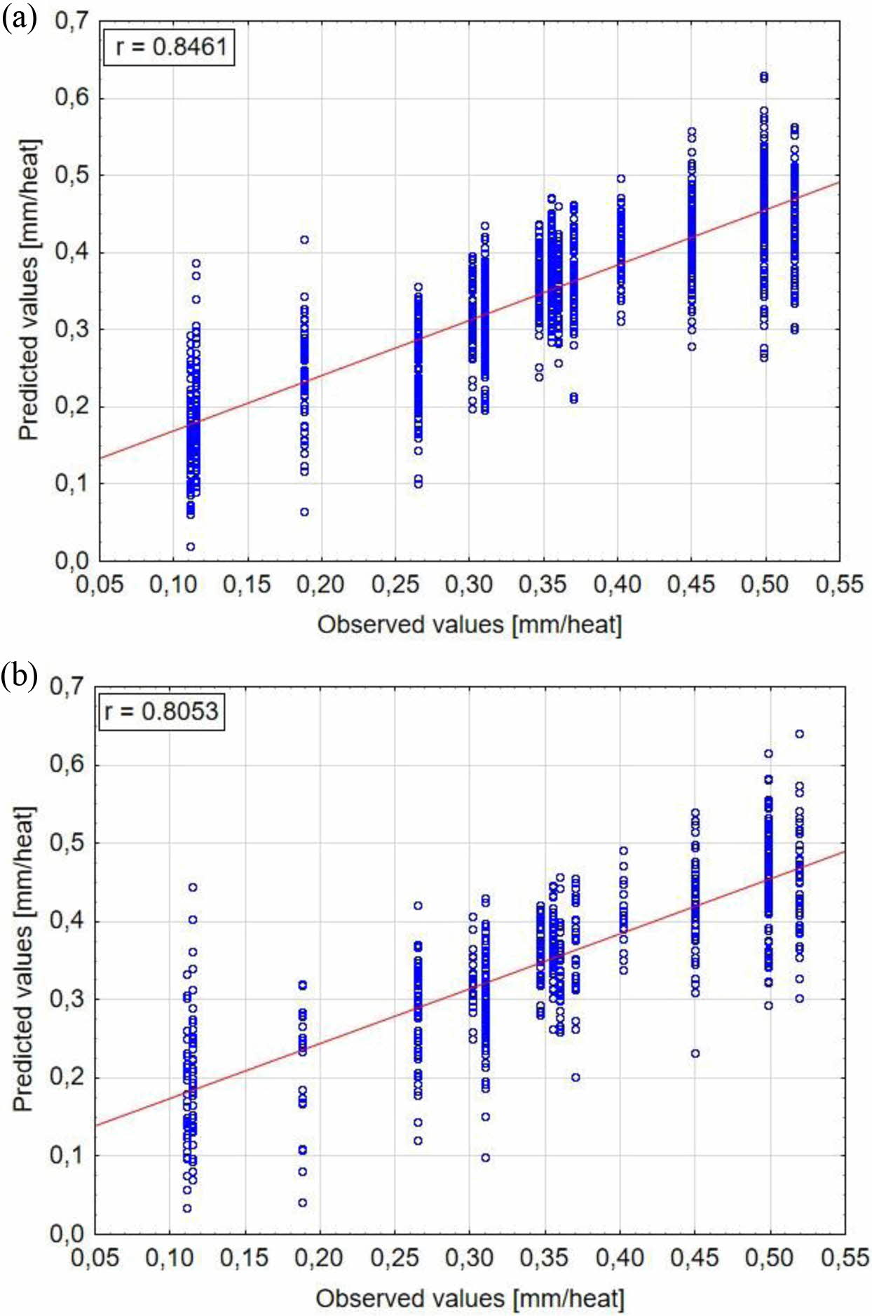
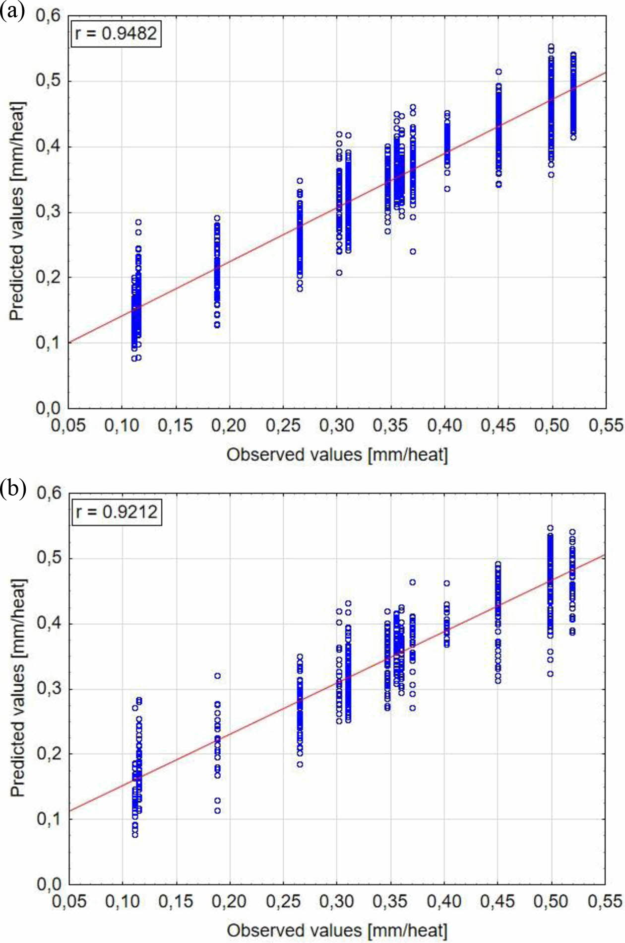
The quality of all models were characterized by calculating different measures of fit for training and testing data. Scatterplots showing observed and predicted values of dependent variable are shown in Figs. 11-14. Fig.12 Fig. 13
A comparison of observed and predicted value results was made with the use of different measures of fit like coefficient of determination R² calculated in accordance to Formula (3) and correlation coefficient calculated in accordance to Formula (4) [18]:



where: γ̅ – mean value of predicted values, y_i – predicted values, x_i – observed values, x mean value of observed measurements.
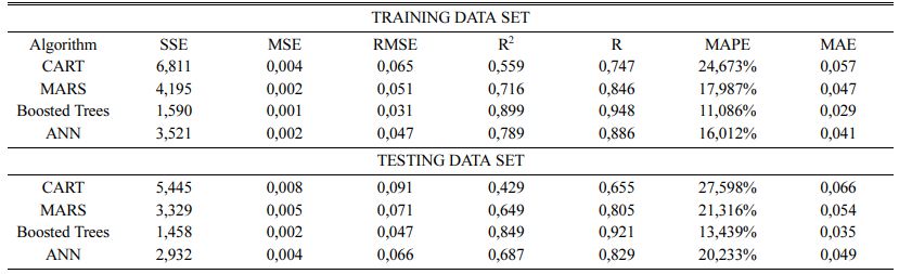
To conduct detailed assessment of models quality and its accuracy for results obtained by the use of different machine learning algorithms SSE (Sum of Squares) values were calculated using Formula (5) [18], where y_i – observed value, γ̂_t - predicted value, n – number of observations.



The MSE (Mean Squared Error) was calculated with the use of Formula (6) which is an absolute measure- ment of model fit.



Another measure of fit calculated for obtained result is RMSE (Root Mean Squared Error)which is a measure of distance between predicted and observed value and it is calculated with the use of Formula (7) as root value of MSE. MSE = 0 means that our data is perfectly fit whereas the lower the RMSE the better the measure of fit. RMSE expressed in the measurement units indicates the average error of selected prediction.



One of the commonly used measurement of fit called MAPE (Mean Absolute Percentage Error)[19] was calculated with the use of Formula 8 and MAE (Mean Absolute Error) calculated with the use of Formula 9.



Table 5 shows a summary of all calculated measures of fit for results obtained in training and testing data sets in applied machine learning algorithms. RMSE is considered as the most authoritative measure of fit. The lowest RMSE value equal 0,031 in training data and 0,047 in testing data is obtained for Boosted Trees algorithm.

• The quality of predictions obtained with evaluated models is not at a satisfactory level. The reason is associated with the quality of initial data set collected during BOF operation, particularly:
- low frequency of lining residual thickness mea- surements,
- missing data in initial data sets for selected variables,
- lack of detailed information about conservation scheme.
The preparation of initial data set for analysis is crucial for the best quality model development.
• The prediction of the best quality characterized by selected measures of fit was obtained with the use of Boosted Trees and MLP algorithms. However, relatively high values of MAPE suggest a necessity of conducting further attempts to predict the wear rate of refractory lining in the slag spout zone of BOF with the use of properly prepared initial data set.
• In accordance to CART, MARS and Boosted Trees models it is possible to inidicate 4 most important variables: hot metal mass (X1), Si concentration in hot metal (X4), scrap mass (X5), oxygen activity (X9), which is confirmed by practical observations connected with industrial experience.
• For increasing the quality of refractory lining wear prediction it is necessary to include a conservation scheme data into the initial data set which will enable the use of mixed models containing both qualitative and quantitative variables (numbers of gunning operations, slag splashing done and slag washing by rocking the vessel).
• It is necessary to conduct a laser measurement of lining thickness just before a converter stoppage.